About MarkInfo

Frequency maps can be constructed for so-called categorical variables. One example is soil moisture, where each sample plot is assigned a soil moisture class. Since the sample plots in the National Forest Soil Inventory are objectively located and therefore regarded as area-representative, the percentage share of each class within a variable can be calculated for a given geographical area.

An area encompassing Sweden’s national boundaries has been delimited within the national coordinate system (Rikets nät), with the southern boundary at 6,100,000 metres and the northern boundary at 7,700,000 metres north of the equator. In the west, the boundary is set at 1,200,000 metres and in the east at 1,900,000 metres east of the Greenwich meridian. Within this defined area, a grid with 25 km spacing between intersection points has been established. For each intersection point, the frequency of the classes of the studied variable has been calculated.

This has been done by including all sample plots within a radius of 40 km from each intersection point. The actual distance of each sample plot to its corresponding intersection point has been taken into account in the calculations, following the principle that the influence of a plot decreases with the square of the distance to the intersection point. In addition, the so-called area factor has been considered, since it varies both by region and as a result of any subdivision of the sample plot.

The area factor represents the area that a sample plot corresponds to when, for example, summing forest land area. In Region 1, located in the interior of northern Norrland, a single sample plot represents a substantially larger area than a plot located in Region 5 along the southern coastal areas. When a sample plot is subdivided, for example by a stand boundary, the area factor must be reduced in proportion to the fraction of the plot remaining. To account for this, the influence of each plot in the calculations is also reduced linearly according to its area factor.
Since the distance between grid intersection points is 25 km and the radius used is 40 km, a single sample plot will typically influence several frequency calculation points, albeit with different weights. This results in a smoothing effect and prevents unrealistic peaks in the final presentation.

In the resulting grid, each intersection point includes not only the percentage values for each class of the studied variable (which always sum to 100%), but also the number of observations.

In the next step, a linear interpolation is performed to create a denser grid with 5 km spacing between intersection points, using the SAS procedure G3GRID. The resulting grid is then plotted using the SAS procedure GPLOT, where each point (with x representing the east coordinate and y the north coordinate) is assigned a colour corresponding to its class when the data are divided into five classes with equal class intervals.

In transition zones near mountains and water bodies, as well as in areas with a low proportion of forest land where sample plot density is low, certain points are removed. A minimum threshold for the number of observations per point is applied. This threshold varies by region, reflecting differences in sampling intensity, which is lowest in Region 1 in the far north and increases southwards, reaching its highest level in Region 5 along the southern coast. The thresholds are set in proportion to the sampling density differences between regions.

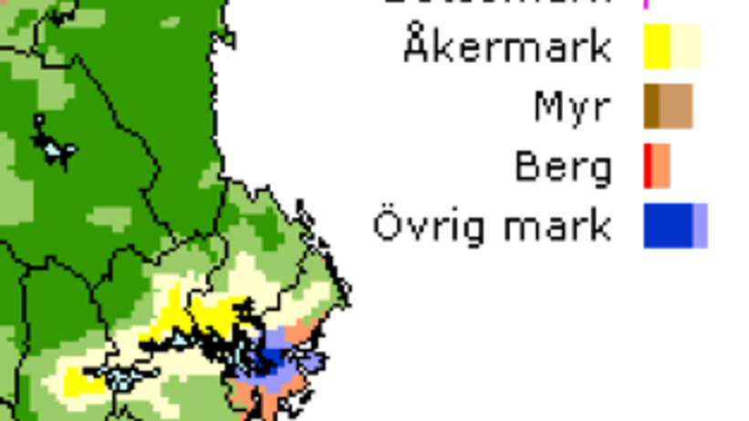
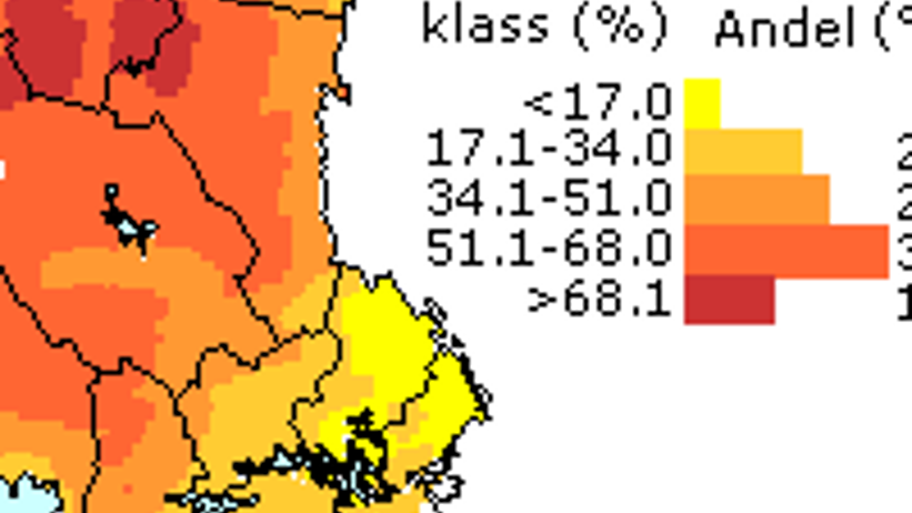
The primary purpose of dominance maps is to provide an overview of the areas in Sweden where a particular class of a variable can be expected to dominate. For instance, if one wants to identify where iron podzols are the most dominant soil type, this can be determined using the frequency matrices that form the basis of the frequency maps.

The approach is to determine, at each grid intersection point, which class has the highest frequency and how large it is in comparison with the next most common class. This makes it possible to rank the intersection points according to the degree of dominance and divide the entire dataset into two equally large groups: one with high and one with low dominance. Each intersection point thus contains information both on which class is dominant and on the dominance class to which it belongs.

The map is produced by assigning different colours to different classes, and by distinguishing strong dominance from weak dominance through variations in colour intensity.

The bar chart accompanying the dominance maps shows the frequency distribution among the different classes, expressed as percentages that closely reflect the actual distribution across the country. The distribution within the dominance classes is also shown in the diagram. 

As for the frequency maps, an area encompassing Sweden’s national boundaries has been defined within the national coordinate system (Rikets nät). The southern boundary is set at 6,100,000 metres and the northern boundary at 7,700,000 metres north of the equator. In the west, the boundary is set at 1,200,000 metres and in the east at 1,900,000 metres east of the Greenwich meridian.

Within this defined area, a grid with 20 km spacing between intersection points has been established. For the variable under study, a weighted mean has been calculated for all sample plots within a radius of 30 km from each intersection point. The weighting factor is based on the product of the maximum distance (30 km) minus the distance between the sample plot and the intersection point, and the area factor of the plot. Consequently, plots located close to the intersection point and with a high area factor (i.e. undivided plots) are given the greatest weight in the calculation of the mean value.

The production of the maps themselves follows the same principles as for the frequency maps.

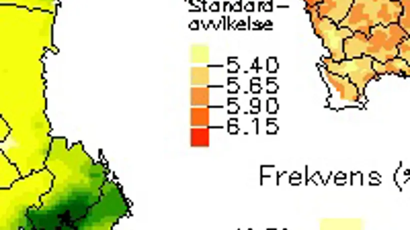
The kriging method is, in brief, based on taking into account the spatial variation of a variable. Compared with direct interpolation of sample plot values, this method provides more reliable estimates of the variable between sampling points. In kriging-interpolated maps, the standard deviation at each point is presented in a separate, smaller map. In addition, a histogram shows the frequency distribution across classes.

Kriging is a geostatistical method used to interpolate values of a given variable at unsampled locations. Unlike conventional “mathematical” interpolation, kriging accounts for the actual autocorrelation present in the collected data. This autocorrelation is described using a so-called variogram. A variogram is a diagram in which the semivariance (i.e. the variance between two points) is plotted against the separating distance between those points. A function is fitted to the points in the variogram, thereby providing a mathematical description of the spatial variability of the variable. A variogram is thus unique to each variable. The fitted function, also referred to as a “model,” is then used in the kriging interpolation. This model forms the basis for the kriging weights assigned to surrounding observations when estimating the value at an unsampled location.

The advantages of kriging compared with other interpolation methods include improved reliability of the estimated values at interpolated points. The distance dependence applied in the interpolation is determined by the shape of the variogram. Kriging also takes into account the spatial distribution of the observations used for interpolation. For example, less weight is assigned to individual points within clusters of closely spaced observations. In cases where two points are aligned, the more distant point is given less influence due to its “sheltered” position relative to the nearer point. In addition to the estimated value, kriging also provides an estimate of the variance (or standard deviation) at each interpolated point.

In the kriging-based maps in MarkInfo, ordinary kriging has been applied (Davis, 1986). This has been carried out on datasets that have been detrended and, in some cases, transformed (log-transformed). The interpolation has been performed on a grid with 5 km spacing, taking into account up to 20 sampled points within a maximum radius of 80 km. The maximum number of points has been selected based on the degree to which the sampling design is systematic or random (Webster & Oliver, 1990). The maximum radius is only reached when interpolating in peripheral areas.

An area encompassing Sweden’s national boundaries has been defined within the national coordinate system (Rikets nät). The southern boundary is set at 6,100,000 metres and the northern boundary at 7,700,000 metres north of the equator. In the west, the boundary is set at 1,200,000 metres and in the east at 1,900,000 metres east of the Greenwich meridian.

Within this area, each sample plot has been assigned coordinates with a precision of 100 metres. A conceptual grid has been overlaid on the defined area, with 25 km spacing between the intersection points. These intersection points also coincide with the corners of topographic map sheets (e.g. Uppsala SW).

For each intersection point, the necessary information for conducting trend analyses has been calculated. The sample plots included in the calculations are those located within a circular area with a radius of 40 km from each intersection point (see figure below).

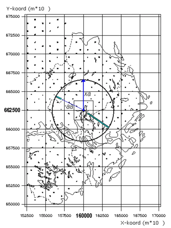
Figure 1. Illustration of the grid with intersection points spaced 25 km apart and the circular area, with a radius of 40 km, within which sample plots are included in the calculations. The thick radial lines illustrate the distance component of the weighting factor. The sample plot located to the south-east of the intersection point receives a high distance weight, whereas the more distant sample plot to the north-west receives a lower weight. The square surrounding the intersection point represents the area (25 × 25 km) displayed in the maps.

Weighting factor

The actual distance of each sample plot to the intersection point it represents in the calculations has been taken into account. This has been done according to the principle that the greater the distance from the intersection point, the less influence the plot should have on the calculation.

Furthermore, the so-called area factor has been considered, as it varies both due to the regional affiliation of the plot and because the plot may be subdivided. The area factor represents the area corresponding to a sample plot, for example when summing the area of forest land. In Region 1, located in the interior of northern Norrland, a sample plot represents a substantially larger area than a plot located in Region 5 along the southern coast. When a sample plot is subdivided, for example by a stand boundary, the area factor must be reduced in proportion to the fraction of the plot that remains.

To account for both the actual distance of each sample plot from the intersection point and the variation in area factors, weighted calculations have been performed. The weighting factor used is defined as the product of the area factor and the maximum distance minus the distance of the plot to the intersection point, divided by 10⁶ to obtain a more manageable scale, as follows: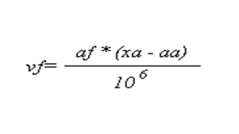

where vf = weighting factor, af = area factor, xa = maximum distance (m × 10⁻¹), and aa = actual distance (m × 10⁻¹), as illustrated in Figure 1.

The weighting factor (vf) thus takes on values in the order of 1 to 80, where plots with higher values carry the greatest weight in the weighted calculations.

Calculated variables – step 1

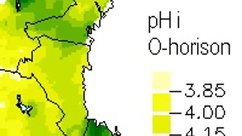
For the trend maps displaying pH in the organic layer, the analyses are based on pH measurements from organic layer samples collected during the periods 1963–72, 1973–75, 1983–87, and 1993–99 (in total more than 62,000 observations). A joint database has been created for further processing.

The first step has been to generate a SAS table which, for each grid intersection point (as described above), contains the weighted (as described above) mean hydrogen ion concentration (transformed pH value), its standard deviation, and the number of observations theoretically contained within a “square” (as defined above). This has been carried out for each intersection point and inventory year.

Calculated variables – step 2

From step 1, approximately 700 “squares” with 25 km sides are obtained, containing the variables hydrogen ion concentration, year, standard deviation, and number of observations.

To ensure well-defined and reliable mean values, squares with fewer than 10 observations are excluded. The same applies if the standard deviation exceeds the mean value.

This results in approximately 600 remaining “squares”, for which the relationship between year and hydrogen ion concentration is tested for each square. An additional requirement is that the number of observations included in each function must be at least 10. The hypothesis is that in those squares where no relationship is found, no change in pH has occurred during the period 1963–1999. 

An example of the relationship between time (expressed in years) and hydrogen ion concentration for a single square is shown in the figure below.

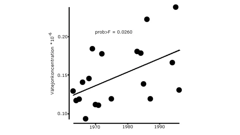
Figure 2. Example of a “square” where the hydrogen ion concentration increases significantly over time during the period 1963–1999.

To illustrate possible changes, as well as their magnitude and rate, further calculations are carried out. The derived functions are therefore used to generate annual estimates from 1963 to 1999 for each “square”.

Maps are then produced by transforming hydrogen ion concentration back to pH, with one map generated for each year. These maps are combined into an animated GIF, which clearly illustrates any temporal changes.

A map showing the probability value for each “square” provides an indication of where in the country any observed change can be considered statistically significant. In addition, a separate map is produced showing the annual rate of change, expressed in hydrogen ion concentration per year.